Machine Learning by Least Squares and Scikit Learn
Prediction of unknown values by making use of historical data is the core of machine learning. As a warm-up to machine learning, let’s work on global warming data to estimate future values in this post. All you need to have is up and running Python environment i.e. Anaconda with Jupyter notebook, with some pip packages installed. Rest is explained in details here 🐧
Discovering the Data
In the link here, you can find the CSV formatted data for Arctic ice level change over the years. Unless you are a scientist in NASA, this values are no different than any other time-series data. As a summary, you can see that the file has Year and All Antarctica columns that we interest in this post.
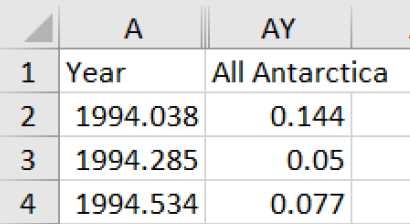
You can start importing the data and Pandas will parse it for you to prepare the tabulated data.
import pandas as pd
dataset_url = 'https://sealevel-nexus.jpl.nasa.gov/data/ice_shelf_dh_mean_v1/ice_shelf_dh_mean_v1_height.csv'
dataset = pd.read_csv(dataset_url)
dataset.head()
If everything worked fine you are supposed to see first few lines of the dataset. We have 72 samples in total which is sufficient for many machine-learning methods but not enough for some others.
Let’s create x and y vectors.
import numpy as np
# Read CSV into table and get (x, y) pairs.
N = dataset.shape[0] # size of input samples
x = np.array(dataset['Year']).reshape([N, 1])
y = np.array(dataset['All Antarctica']).reshape([N, 1])
points = np.hstack([x, y])
Creating the Model
Least Squares Estimation
This technique is quick and dirty. Its purpose is finding a line, or model, that makes the minimum error in sum of square of difference with the real data samples. More clearly, if you have 3 x-y pairs in 2 dimensional space i.e. [[1, 0], [2, 3], [3, 2], [4, 5]], least squares regression will put a line passes between all the points.
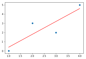
This post is aimed to evaluate different ways of predicting values so I wont deeply focus on the mathematical foundations. The Generalized Least Squares equation for third-order model is given below. Here x is vector of years and y is vector of melting ice level. What we search for is the solution set of m coefficients that will be used for creating the polynomial model.

For further details on how we came up with this, refer to 2.3 Generalized Least Squares in Shiavi’s book.
Solve the Least Squares Regression by Hand
To solve the above equation for linear model parameters, we should create the matrices from the dataset.
# Calculate power series sums.
x0 = np.sum(x**0)
x1 = np.sum(x**1)
x2 = np.sum(x**2)
x3 = np.sum(x**3)
x4 = np.sum(x**4)
yx0 = np.sum(y * x**0)
yx1 = np.sum(y * x**1)
yx2 = np.sum(y * x**2)

# Create 3rd order model matrices.
A = [[x0, x1, x2], [x1, x2, x3], [x2, x3, x4]]
B = [[yx0], [yx1], [yx2]]
Obtain Model Coefficients
Simply solve the LS equation by matrix inversion and matrix multiplication. As soon as we have more independent data points that the number of unknown parameters, there exists a solution.
import numpy.linalg as lin
M = np.matmul(lin.inv(A), B)
The degree-two polynomial coefficients are found as below.
[[-5.48765643e+03],
 [ 5.49213398e+00],
 [-1.37413749e-03]]
Simulate the Estimated Curve
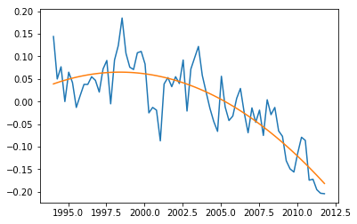
To visualize the result, we can create y_estimated, by hand again.
import matplotlib.pyplot as plt
y_estimated = x**0 * M[0] + x**1 * M[1] + x**2 * M[2]
plt.plot(x, y, x, y_estimated)
plt.show()
Prediction of Future Values
This may seem like it will diverge soon in near future. Let’s make a prediction for year 2020 to see.
y2020 = 2020**0 * M[0] + 2020**1 * M[1] + 2020**2 * M[2]
Ice melting level by the beginning of 2020 is predicted as -0.576 which looks reasonable. For people who are not convinced by this, simply use the same steps for second-order model (simply drop the third line of the matrices and obtain a straight line that is likely to pass close to the average of values.
RMS Error
To see the overall performance of the fit, we can simply take root-mean-square of the error.
rmse = (np.sum((yest - y) **2) / len(y)) ** 0.5
And the result is 0.047179935281228005.
Easier Approach with PolyFit
The above part is for understanding how generalized least-squares work. Now we can use pythonic way to get the same result with less pain. Here is how it works.
m = np.polyfit(x.flatten(), y.flatten(), 2)
y_estimate = np.polyval(m, x.flatten())
plt.plot(x, y, x, y_estimate)
plt.show()
Compare the Results
Coefficients of the model we created with polyfit(…) are given below. (Note that in reverse order.)
[-1.37411264e-03 5.49203444e+00 -5.48755675e+03]
We can observe the RMS error of 0.9580719383950538 in polyfit is worse than manual solution above. This is caused by precision difference in the computations.
Higher Order Model
Now only because we can do it, let’s build fifth-order (degree-four) model by changing the first line. Resulting model coefficients are [-3.62567002e-06 2.89804373e-02 -8.68672643e+01 1.15725246e+05 -5.78142126e+07] and the curve is shown below. RMS error of 0.9602434264337656 is not improved.
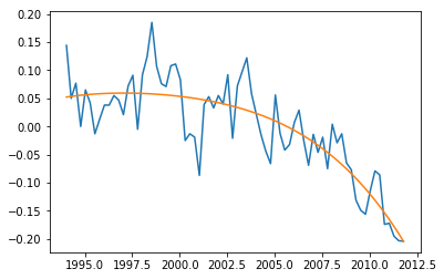
The prediction for 2020 is -1.094 and slightly differs than the previous prediction. Since higher order models reduce regularization and are vulnerable to over-fitting, it is better to proceed with a second or third order model.
Linear Regression in Scikit Learn
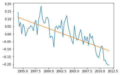
Alternatively, Scikit provides LinearRegression() that we can evaluate on this simple problem. There are not many details to discuss here since it is quite simple. Lets see the results below.
from sklearn.linear_model import LinearRegression
regressor = LinearRegression()
model = regressor.fit(x_train, y_train)
regressor.predict(np.array([2020]).reshape([-1, 1]))
y_predicted = regressor.predict(x)
plt.plot(x, y, x, y_predicted)
plt.show()
The slope and y-intercept are [-0.012416 24.86813385] and 2020 prediction is -0.212. Finally the RMS error is found as 0.05767110113039651 with the code below.
from sklearn.metrics import mean_squared_error
rmse = mean_squared_error(y, yest)**0.5
Support Vector Machine
Another approach to this problem is using SVM regression. If the concept is unfamiliar, check this first.
Discovering Hyper-Parameters
Support Vector Machines need several parameters such as C, the regularization factor (small values ignore more disturbance); epsilon, the penalty tolerance value (greater values disregard more of outlier); and model type such as RBF or polynomial.
Use Grid Search Cross-Validation for Hyper-Parameter Tuning
Scikit Learn GridSearchCV(…) picks the best performing parameter set for you, using K-Fold Cross-Validation. It simply divides the dataset into i.e. 3 randomly chosen parts and trains the regression model using 2 of them and measures the performance on the remaining part in a systematic way.
from sklearn.model_selection import GridSearchCV
from sklearn.svm import SVR

# Best setting for each parameter will be chosen
parameters = {
    'C': 10.0 ** np.arange(-4, 1),
    'kernel': ['poly', 'rbf', 'sigmoid'],
    'epsilon': 10.0 ** np.arange(-4, 1),
    'degree': [2, 3, 4],
}

# Create SVM Regressor
regressor = SVR(max_iter=1000000)

# Run grid search with 3-fold cross-validation
cv = GridSearchCV(regressor, parameters, cv=3)
cv.fit(x, y)
To see the best parameters, check cv.best_params_ and for the best score, check cv.best_score_. I got {‘C’: 1.0, ‘epsilon’: 0.01, ‘kernel’: ‘rbf’} and the best score is -2.142. This negative score implies something went wrong. Really, in this example dataset, we have not enough values to generalize and that is obviously the problem. But let’s see the performance of this model which is likely an over-fit.
Test The SVR Model
Now we the split dataset into test and training parts, fit the SVR model to training set and test with all data.
from sklearn.model_selection import train_test_split

# Split data, 2/3 for training and 1/3 for test
(x_train, x_test, y_train, y_test) = train_test_split(x, y, test_size=0.33)

# Apply the best parameters to the regressor
regressor.set_params(**cv.best_params_)

# Fit the model to training data
regressor.fit(x_train, y_train)

# Predict results for both train and test data
y_predict_train = regressor.predict(x_train)
y_predict_test = regressor.predict(x_test)

# Plot
plt.plot(x, y)
plt.scatter(x_train, y_predict_train, c='r')
plt.scatter(x_test, y_predict_test, c='k')
plt.show()
Results for SVM Regressor
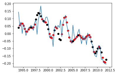
The result is given in the plot. Red dots are the training set while the black ones are the test set. We can clearly comment on this plot that the model regularization is low and it memorized the monthly variations rather than overall annual trend. Predicted 2020 melting level is 0.001 which is even positive.
Discover other tools in sklearn library and evaluate different methods such as MLPRegressor(…) which uses multi-layer neural-network behind the scenes. Scikit Learn is well-documented on the official page.
Summary
In this post, I used very limited data and only single dimensional input since the aim is teaching how to catch a fish rather than catching a fish. Until next time 🐟🐠🐡
